Kalman filtering and jitter
First blog post! It’s gotten rather technical - a bit more than initially aimed for - and if we discuss things in depth, we might as well go for a more academic style. I hope it’s sufficiently clear, and if not, be sure to share in the comments. Enjoy the read!
Introduction
The Kalman filter is one of the most widely employed estimators in robotics and other fields. Its robust capability to filter out noise, combined with its relative ease of tuning and extensive explainability, positions it as a straightforward choice. Consequently, its workings and implementation are extensively covered in numerous engineering books, as well as online such as kalmanfilter.net.
A subject rarely covered, however, is how to handle measurement timing noise or jitter. While the standard Kalman filter does take into account measurement noise (in the form of a covariance matrix), it still assumes that this measurement was taken at exactly the reported time instant \(t\). This despite timing noise being a common occurrence in many real-life systems, especially robots. Of course, it is preferable to eliminate this uncertainty at its source, however accomplishing that is often not straightforward. For instance, because the measurement is processed by a third-party module. A makeshift solution is to increase the overall measurement covariance. However, as this post will discuss, there are two other methods which tackle this challenge more effectively.
The first method addresses measurement time uncertainty by incorporating it into the innovation covariance matrix. It assumes that the timing error follows a known standard normal distribution and projects this uncertainty onto the innovation covariance along the state time derivative, enabling the derivation of a suitable Kalman gain. The second method takes this concept further - essentially taking the limit of timing uncertainty to infinity - and as such delivers a fully measurement time-invariant Kalman correction: the time at which the measurement was taken has negligible influence on the applied correction, assuming sufficient local linearity.
This blog post will discuss both methods, but, before going into details, we will first introduce the used symbols, and an example system such that the two methods can be evaluated with an application example.
Math terms
Here’s an overview of the symbols we will use:
| Symbol | Name |
|---|---|
| \(\mathbf{x}\) | State |
| \(\dot{\mathbf{x}}\) | State time derivative |
| \(\mathbf{P}\) | State covariance |
| \(\mathbf{z}\) | Measurement |
| \(\mathbf{v}\) | Measurement noise |
| \(\mathbf{R}\) | Measurement covariance |
| \(\mathbf{H}\) | Measurement sensitivity |
| \(\mathbf{S}\) | Innovation covariance |
| \(\sigma_t^2\) | Measurement timing variance |
The state time derivative \(\dot{\mathbf{x}}\) deserves some further explanation. While almost always a Kalman filter is implemented as discrete, here this derivative points to the time derivative of the continuous counterpart of the state vector.
Example system
To illustrate these methods, we will apply them to a straightforward system - an unmanned ground vehicle (UGV) with mecanum wheels operating in a room. The UGV can move horizontally (x and y axes) and due to its built-in compass and control system, it maintains a constant heading. (Allowing it to rotate is more realistic, but would add unnecessary complexity.) This system has four states, two positions and two velocities. The UGV is equipped with an accelerometer, measuring x- and y-acceleration, and these measurements propagate the filter. Additionally, a camera on the UGV observers a marker on the ceiling and outputs a position observation \(\mathbf{z}\). The camera is a simple webcam which lacks precise timestamping, leading to some jitter in these position measurements.
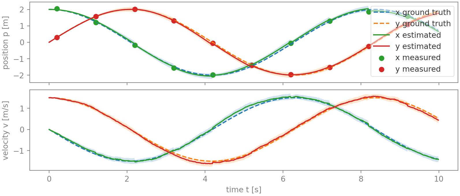
In this example, the UGV drives a perfect circle of radius 2 m around the origin at a velocity of 1.5 m/s. The Kalman filter is propagated at 100 Hz and corrected at 2 Hz. The following measurement noise is present (standard deviations):
| Sensor | Measurement | Symbol | Amount | Unit |
|---|---|---|---|---|
| accelerometer | acceleration | \(\sigma_a\) | 0.5 | m/s² |
| camera | position | \(\sigma_p\) | 0.05 | m |
| camera | position timestamp | \(\sigma_t\) | 0.15 | s |
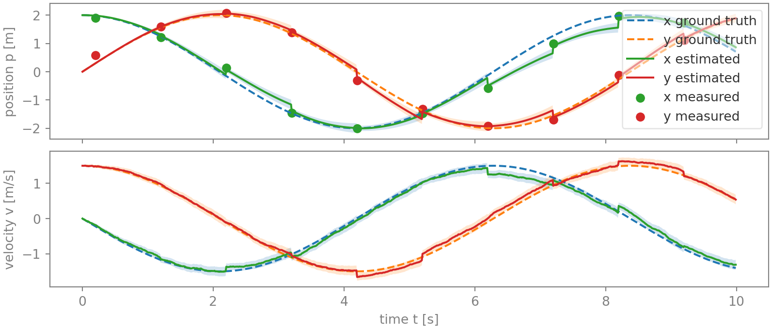
The figures below graph the position and velocity estimates, together with their two-sigma uncertainty in shaded, and the position ground truth and the camera observations. In the first figure, no timing noise is present, while in the second, minor timing noise was added to the camera observations. Both were derived using simulation, and the acceleration and position noise in the two is identical.


While the Kalman filter delivers an admirable estimation in both cases, in figure 2 the state estimate has become noticeably more jumpy. Notice in particular the jumps for the x-position between 6 and 8.3 s. Also worrying is that for several samples, the error is larger than the two-sigma uncertainty range, indicating that the state covariance \(\mathbf{P}\) is underestimating the error magnitude. This is not surprising, giving that the actual position measurement noise is larger than expected due the additional timing noise.
Let’s see whether we can improve on this baseline!
Method 1: Time error projection
Theory
The key issue is that, in its standard form, the Kalman filter is not aware of the timing noise. A timing error of duration \(\Delta t_r\) implies that a measurement \(z\) was not taken at time \(t\) but at time \(t - \Delta t_r\). To obtain the resulting error \(\Delta \mathbf{z}\), we approximate it with a first-order Taylor series:
\[\begin{align*} \mathbf{z} &= \mathbf{H} \, \mathbf{x} + \mathbf{v} \\ \Delta \mathbf{z} \approx \dot{\mathbf{z}} \Delta t_r &= \frac{\partial}{\partial t} \left( \mathbf{H} \, \mathbf{x} + \mathbf{v} \right) \Delta t_r = \mathbf{H} \, \dot{\mathbf{x}} \, \Delta t_r \end{align*}\]In practice, \(\Delta t_r\) is unknown, only its distribution, in the form of its standard deviation \(\sigma_t\), is known. Its effect is therefore expressed as a covariance. The standard Kalman filter calculates the innovation covariance as
\[\mathbf{S} = \mathbf{H} \mathbf{P} \mathbf{H}^\mathsf{T} + \mathbf{R}\]and to account for the uncertainty resulting from the unknown timing error, we add the term \(\dot{\mathbf{x}} \sigma_t \otimes \dot{\mathbf{x}} \sigma_t\) projected into observation space. This addition modifies the innovation covariance to
\[\mathbf{S}' = \mathbf{H} \, \left( \mathbf{P} + \dot{\mathbf{x}} \sigma_t \otimes \dot{\mathbf{x}} \sigma_t \right) \, \mathbf{H}^\mathsf{T} + \mathbf{R}\]Graphical interpretation
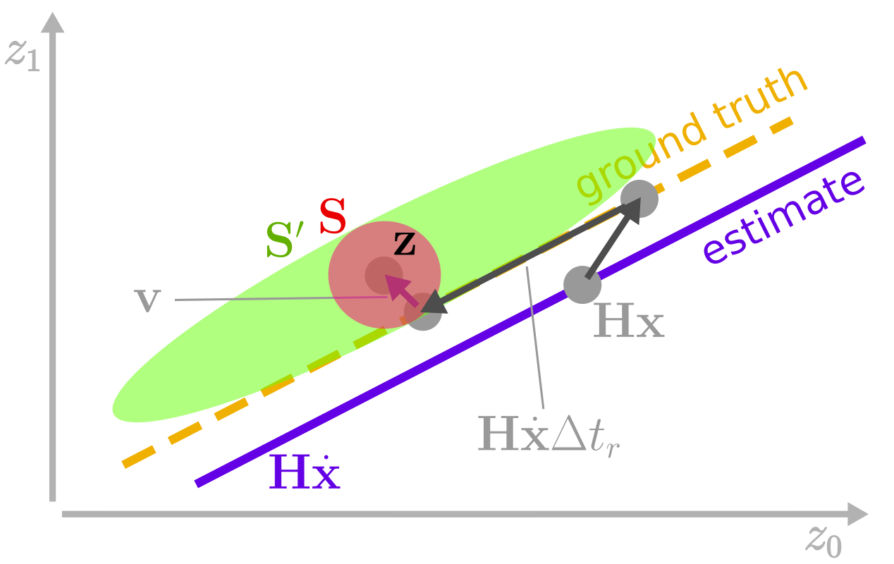
Before delving into the simulation results, let’s visualize the errors in the system, as shown in figure 3 below. Take note of how adding the additional term causes the measurement uncertainty ellipse to grow from the default \(\mathbf{S}\) to the adjusted, elongated \(\mathbf{S}'\). The latter is elongated along the observation derivative \(\mathbf{H} \, \dot{\mathbf{x}}\). For completeness, the measurement noise \(\mathbf{v}\) is also included.

Application example
Inserting this minor additional term into the simulation greatly changes the estimate, and for the better. As figure 4 below shows, all the large jumps are gone, and the uncertainty range now encompasses the actual error. Although this estimate doesn’t match the precision achieved in a system without timing noise, it comes remarkably close — particularly for the velocity, which is not even directly observed.

Method 2: Measurement time-invariant correction
What if… we could totally disregard time? A shortcut would be to greatly overestimate \(\Delta t_r\), and while numerically that gets close, taking the limit to infinite timing uncertainty provides an interesting academic exercise. Let’s see how we can do this.
Theory
The basic idea is that we project the observation onto a new space orthogonal to \(\mathbf{H} \dot{\mathbf{x}}\), and execute the correction as if the observation occurred in this space instead of the original measurement space. Let \(\mathbf{Z}\) of size \((n_z-1) \times n_z\), with \(n_z\) the length of \(\mathbf{z}\), be a projection matrix that projects from the original observation space to this new space. (Therefore, due to the new space being orthogonal to \(\mathbf{H} \dot{\mathbf{x}}\), \(\mathbf{Z} \, \mathbf{H} \dot{\mathbf{x}} = \mathbf{0}\).)
Projecting the innovation to this orthogonal space is easily realized with \(\boldsymbol{\nu}_Z = \mathbf{Z} \, \boldsymbol{\nu}\). The accompanying innovation covariance also has to be projected:
\[\mathbf{S}_Z = \mathbf{Z} \, \mathbf{S} \, \mathbf{Z}^\mathsf{T}\]Of course, handling this different observation requires minor modifications to the Kalman gain and the covariance update. Both can be seen as using a modified observation matrix \(\mathbf{H}_Z = \mathbf{Z} \, \mathbf{H}\), such that the Kalman correction is handled as normal, just in a different space.
Interpreting this visually, it is as if we would look to the observation in figure 3 along the \(\mathbf{H} \dot{\mathbf{x}}\) axis, resulting in any timing error being projected out, and only the orthogonal, time-invariant errors remaining.
Application example
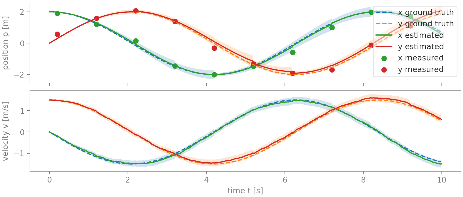
Figure 5 graphs the result of applying the position measurements this way. Compared with the previous method, some errors have become even smaller (those between 6 and 8.2 s for the x-position), while others have grown slightly (4.5 to 6.2 s for the y-position).

System observability
To finish, let’s briefly touch on system observability. Note in figure 5 how the covariances (shaded areas) vary over time. For the positions, they increase most rapidly when the position varies rapidly, and, on the other hand, reduce quickly when the position curve goes flatter. Qualitatively, this an expected result of observing the system only orthogonal to its time direction: the more rapidly a position estimate changes (compared to the other position estimate), the less observable it is because a particular time uncertainty implies a (relatively) larger position error. This is also reflected by the change in the observation matrix from \(\mathbf{H}\) to \(\mathbf{H}_Z\) - especially the latter having one row less - which implies reduced observability. This reduced observability is not an issue as long as this time direction - i.e. the state time derivative - varies over time, which is the case in this example, as well as in many real-life systems. Also, for that reason the first method is usually preferred because it continues to observe the system in the time direction, just with a lower, more appropriate weight.
Conclusion
In conclusion, this blog article explores two approaches to handle timing noise in Kalman filters. A simulation of a virtual UGV demonstrated that both methods filter out the jitter effects almost completely, confirming that these methods effectively address jitter.
The first method incorporates the uncertainty of the measurement timing into the innovation covariance matrix, resulting in an adjusted Kalman gain. The second method goes a step further by assuming the timing uncertainty as infinite, yielding a measurement time-invariant Kalman correction. To realize this, this second approach projects observations onto a new space orthogonal to the state time derivative.
What are your thoughts on this? Did you already encounter timing issues, and if so, how did you resolve them? Share in the comments! Any questions are welcome as well, of course.
Enjoy Reading This Article?
Here are some more articles you might like to read next: