Vehicle Dynamics Sim: accurately and easily simulate actuation limits
Update 2026-02-02: had a blast presenting this at FOSDEM, thanks video team for the recording (10 min)! Also check out my related blog post.
Why your navigation controller works in simulation yet fails on hardware
You’re carefully developing your new robot, setting up and tuning Nav2. It drives around beautifully in Gazebo, confidently exploring new environments. After several weeks, you put the code on your Turtlebot. The result: a violent oscillating mess, motors screeching. What went wrong? Checking the code, everything looks fine. Then it must be the hardware? No, the answer is simple: the simulation was way too perfect, and the real world behaves slightly differently, invalidating the tuning. This is known as the Sim To Real Gap.
Once we look into the simulator’s implementation, the reason for this gap becomes clear: it assumes zero-latency communication, infinite torques, feedback controllers operating on perfect velocity measurements, and other fairy tales. As a result, what runs fine in simulation barely works (if at all) once put on the real platform. This greatly limits the value of simulation in the development process.
Though many simulators can be extended to support these non-idealities, this takes considerable time and effort, especially as one also has to check for correctness. What started as a small task on development tooling quickly grows into a veritable side quest, diverting resources from the actual task.
Other common pain points
Next to the accuracy problem, there’s also a usability aspect. Simulators tend to be difficult to configure and integrate. For example, to use Gazebo with ROS 2, one has to configure it by putting parameter values in the URDF, and usually also some lines in the world environment. If something’s wrong—good luck, as many failures are silent, and documentation is sparse (a dive into the source code tends to be your best friend). Also, one has to configure and launch a message bridge, because Gazebo uses its own message transport system. Finally, there’s the issue that many simulators are computationally heavy, to the point that the nodes you’re actually interested in get starved from CPU.
All in all, with so many things to fix, one starts to wonder whether it’s more time efficient to write something from scratch.
A new simulator
To address this, I decided to focus on realistic actuator modelling, ease of configuration and efficient computations. The result: the ROS package vehicle_dynamics_sim.
Key features:
- Measurable parameters: All values directly observable in real systems (no abstract physics parameters or inverse modeling required).
- Elaborate actuator modeling (dead time, low pass effect, acceleration and velocity limits, etc.) as well as localization modeling (odometry random walk, measurement noise).
- Single YAML configuration: Fully configured through ROS parameters; no URDF editing required.
- 100% native ROS 2: straight pub-sub, no abstraction layers or bridges.
- Lightweight: <500 LOC main file (vehicles.cpp), <15% single-core CPU usage, launches in <1s.
Nice to haves:
- Compatible with Nav2, example config and launch files.
- Wall clock mode: just follows the wall clock progression, very close to how real hardware behaves. No need to use
use_sim_clock(though we do support that, if you need it). - Many vehicle types included: bicycle model (Ackermann), differential and omni, and for the bicycle model we support the four variations (steering rear/front and drive rear/front).
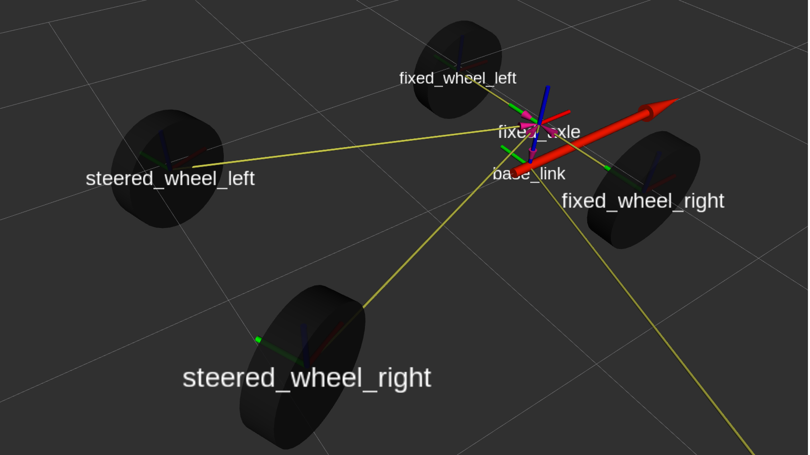
- Robot model visualization (URDF) generated on the fly based on the set ROS parameter values. (This simulator relies on RViz for its viewport.)
Technical deep dive
Actuator dynamics matter
Your trajectory controller is actually controlling a second-order system (or higher), not the simple kinematic model often found in the controller’s documentation. You might think: “Sure, there’s a delay, but the robot still gets there eventually, right?”
Well, these delays often have more significant effects than expected:
- Phase lag kills feedback loops: Your controller sees an error and commands a correction. But that correction takes 100 ms to happen. The controller, not knowing this, sees the error persist and commands more correction. Now you’re overcorrecting, and the oscillations begin, because the delay ate through the entire stability margin.
- Rate limits create saturation: Your MPC controller computes the optimal velocity profile assuming it can change steering angle instantaneously. Your steering actuator maxes out at 2 rad/s. Now your “optimal” trajectory is impossible, and your tracking error explodes in every corner.
You can tune down your controller to make it stable even without modeling actuator dynamics, but that means sacrificing performance on the real platform just to match simulation behavior. These aren’t edge cases or manufacturing defects - they’re fundamental characteristics of how actuators work, and importantly, these dynamics are completely predictable. Below, watch what happens when we ask both models to track a trajectory with several velocity changes:
What we simulate
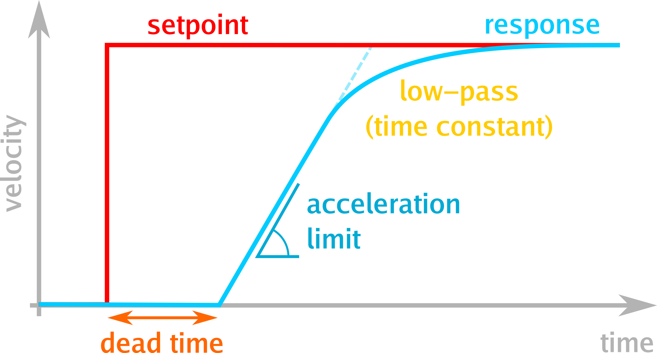
The simulator models the following dynamics for the drive actuator, illustrated schematically in the figure below:
- dead time: The duration it takes for the signal to have any physical effect. This is usually a combination of delays from serial transmissions, layered control loops, and motor driver limiters. In well-designed systems, this delay is negligible (milliseconds); in practice, however, even expensive systems with cascaded controllers often have delays of 200 ms or worse.
- velocity limits: Provided for completeness, usually not relevant. (As taking care of them in the controller is self-evident.)
- acceleration limits: Accelerating a vehicle requires the motor to exert a torque, which requires current. Motor controllers limit this current amplitude to avoid damaging the motor and battery, resulting in finite platform acceleration. (Wheel slip also plays a role, but the electrical limits usually dominate.) While rarely an issue during normal acceleration, these limits become critical when simulating obstacle avoidance and braking, where deceleration is also limited. Acceleration limits are often the dominating factor in emergency stops and collision avoidance scenarios, making them safety-critical for autonomous systems. Controllers that assume instant deceleration will attempt dangerously tight maneuvers that are physically impossible.
- low pass effect: Motor controllers don’t apply full force for every small measured disturbance—that would be wasteful given the constant measurement noise. Instead, they react proportionally to the error (P-controller) and ramp up on persisting errors (I-controller). The resulting vehicle response is well described by a first-order low pass function.

The steering actuator follows a similar pipeline, though limited to position and velocity constraints only. Acceleration limits are not modeled for steering, as their effect is typically dominated by the velocity limits. (If your application requires steering acceleration limits, please open an issue.)
Measurable parameters
Particular care went into making the models not just accurate, but also easily configurable: for example, where other simulators ask for the PID parameters of the motor driver, the vehicle mass, and indirectly the wheel radius, this new simulator condenses all this down into a single parameter— a first-order low pass filter time constant. For a given real-life robot, measuring this time constant is a matter of minutes (apply a step reference and observe the curve in PlotJuggler).
Here’s a comparison table that illustrates the reduction in complexity:
| Traditional Simulator | vehicle_dynamics_sim |
|---|---|
| Motor inertia: 0.05 kg⋅m² | Time constant: 0.12s |
| Gearbox ratio: 20:1 | Max acceleration: 2.5 m/s² |
| Motor KV: 320 rpm/V | |
| Controller P: 0.8, I: 0.2 | |
| Wheel radius: 0.15 m | |
| Mass: 45 kg |
Result: 6 parameters → 2 observable parameters
URDF from YAML
Traditional simulators require separate URDF or SDF files for robot description, which creates two challenges. First, controller developers need to test across multiple vehicle configurations (front-wheel vs rear-wheel steering, different wheelbases, etc.), requiring either multiple URDF files or complex parametrization schemes. Second, URDF-based approaches force simulators to derive vehicle motion from contact dynamics between wheels and ground, adding computational overhead without improving fidelity for normal driving scenarios.
For the RViz visualization, vehicle_dynamics_sim generates the URDF programmatically from ROS parameters. Change wheel_base: 2.7 in your YAML and the visualization updates automatically. No duplicate configuration, no sync issues, no XML wrestling.

Localization realism
Real robots don’t have perfect localization. They have two distinct error sources:
Odometry drift accumulates with distance traveled— wheel slip, encoder noise, and IMU drift all compound into a random walk error. Your odometry frame slowly drifts away from ground truth. Apart from this slow drift, though, noise is usually low.
Map localization (GNSS, SLAM, AMCL) provides bounded but noisy corrections. These measurements have their own characteristics, such as GNSS and SLAM loop closure jumps and particle filter convergence. In general, the map localization estimate is noisy.
vehicle_dynamics_sim models both error sources via the standard three-frame model (map → odom → base_link, REP 105). Drift rates and measurement noise can be configured to match specific sensor suites, providing realistic localization inputs for the navigation stack. This matters because controllers designed assuming perfect localization often fail catastrophically when facing realistic sensor noise, unable to distinguish genuine tracking errors from localization uncertainty.
Expected use cases
This simulator was developed with three key use cases in mind. The first is trajectory following controller tuning. Tuning controllers such as Nav2 MPPI and RPP tends to be a time-consuming hassle requiring access to the real platform. With the package vehicle_dynamics_sim, one only has to use the real platform once (to derive key parameters such as actuator dead time and acceleration limits) and subsequently one can execute most of the tuning in simulation. Though still not as true to reality as the real platform, simulation has other strengths, for example the ability to run parameter sweeps to obtain the perfect tuning by brute force.
The second envisioned use case is in CI/CD pipelines for robot navigation code - fast, reproducible tests without the Gazebo overhead and set-up complexity. Because of the increased accuracy, testing with vehicle_dynamics_sim should also catch more behavioral bugs.
The third use case is teaching and learning. This simulator is ideal for understanding vehicle dynamics and controller behavior without requiring expensive hardware. Students and researchers can experiment with different vehicle configurations, observe how actuator dynamics affect controller performance, and develop intuition, all from their laptop. The lightweight nature means it runs well even on modest hardware, and the visual feedback in RViz makes the learning process immediate and tangible.
It’s important to note the simulator’s scope limitations. It does not model collisions, terrain interactions, or sensors beyond localization. Movement is restricted to 2D planar motion. These design choices reflect the simulator’s focus: complementing full-featured physics engines like Gazebo and O3DE rather than replacing them.
Conclusion
The sim-to-real gap doesn’t have to be a development bottleneck. By focusing on the dynamics that matter most—actuator response and localization— vehicle_dynamics_sim provides a middle ground between perfect kinematic simulation and computationally expensive physics engines.
It won’t replace Gazebo for sensor simulation or collision detection, but for controller development and testing, it offers something valuable: simulation that behaves like your hardware actually does. And, no less important, with it being lightweight to run and easy to configure, usage should be a breeze.
Try it out, tune your Nav2 stack, or integrate it into your CI pipeline. The code is open source (MIT license), contributions welcome, and I’d love to hear how it works for your robot!
Enjoy Reading This Article?
Here are some more articles you might like to read next: