Sensor fusion: be sure of uncertainty

Intro

In case you’ve dabbled in state estimation, there’s a good chance you already encountered the following story: selected some sensors, picked an algorithm (usually Kalman or LQE), spent significant time on implementation and debugging, and then came to the conclusion that the resulting estimate is too noisy. Iteration, trying out other sensors and filter configurations, eventually made for a satisfying result, at the expense of lots of time spent coding and setting up experiments.

Now, here’s the thing: one can gather 90 % of those design insights with just a fraction of the implementation work, and even omit running the filter (in simulation or real-world) entirely. That requires a few targeted short cuts, and this article shows how.

---

To discuss the approach, we’ll go through the design of an estimation system for an autonomous multirotor landing on a visual marker. The used four-state Kalman filter is a simplified version of the one I developed for my master’s thesis.

After a brief discussion of the challenge at hand, the first step is to write out the system matrices. Thereafter we cover the covariance matrices, including translating the discrete measurements to continuous. The final step is to evaluate the relation of sensor noisiness on the state estimate covariance to find out what sensing system improvements will increase performance most effectively. In particular, we’ll see how influential the marker observation rate is, and whether it’s the camera, the gyro or the accelerometer that are to be improved.

Math terms

Key used symbols (lowercase for vectors, uppercase for matrices):

The challenge: autonomous multirotor landing localization

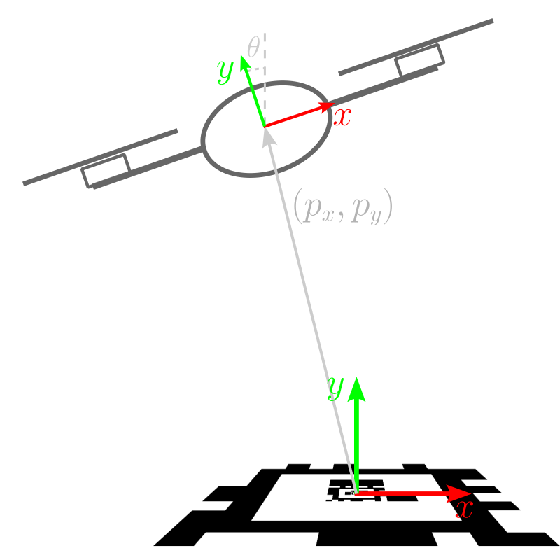
Figure 1 illustrates the challenge: a drone flies above the marker, keeping position while descending. Ground effects and increased turbulence make this situation challenging, and the feedback control system requires a solid source of where the drone finds itself above the marker - it requires a state estimate.

The state vector \(\mathbf{x}\) contains the kinematic state of the drone - position and velocity - as well as a bias term for the gyro (the accelerometer x-axis bias is omitted because of its poor observability):

\[\begin{align*} \mathbf{x} &= \begin{bmatrix} p_x & \theta & v_x & b_\omega\end{bmatrix}^\mathsf{T} \\ \mathbf{u} &= \begin{bmatrix} \omega & a_x \end{bmatrix}^\mathsf{T} \end{align*}\]

As sensor we have at our disposal an IMU (gyro + accelerometer) and a camera that observes the marker. The IMU provides angular velocity and linear accelerations, combining up to the propagation vector \(\mathbf{u}\). On the other hand, the marker detector delivers measurements \(\mathbf{z} = \begin{bmatrix} z_x \end{bmatrix}^\mathsf{T}\), we get the relative position of the marker (no orientation - we’ll analyze the impact of that later). The marker lies at the origin.

The filter: limited design

System matrices

Now, instead of designing and coding up Kalman filter that handles this challenge in full, we’ll limit ourselves to writing out the system matrices and apply the following simplifications:

• 1D instead of 3D. Two instead of 6 DoF, and no quaternions.
• Linear instead of extended. We select one representative state and linearize while modelling.
• Continuous. All sensing is converted from discrete, negating the need to handle sensor synchronization.
• Constant input covariances. As the system operates in a particular representative situation, \(\mathbf{R}\) and \(\mathbf{Q}\) are kept constant, allowing to use LQE instead of a full Kalman filter. What counts is information - not implementation.

In this case, we’ll choose the representative state to be somewhere exactly above the marker. As a result, sines and cosines drop away. For completeness, these are the three system matrices derived after applying the above (with \(g\) = 9.81 m/s²):

\[\newcommand{\gz}[0]{\color{grey}0} \begin{align*} \dot{\mathbf{x}} &= \mathbf{A} \, \mathbf{x} + \mathbf{B} \, \mathbf{u} \\ &= \begin{bmatrix} \begin{matrix} \gz & \gz & 1 & \gz \\ \gz & \gz & \gz & -1 \\ \gz & -g & \gz & \gz \\ \end{matrix} \\ \color{grey} \mathbf{0}_{1 \times 4} \end{bmatrix} \cdot \begin{bmatrix} p_x \\ \theta \\ v_x \\ b_\omega \end{bmatrix} \, + \, \begin{bmatrix} \color{grey} \mathbf{0}_{1 \times 2} \\ \mathbf{I}_{2 \times 2} \\ \color{grey} \mathbf{0}_{1 \times 2} \\ \end{bmatrix} \cdot \begin{bmatrix} \omega \\ a_x \end{bmatrix} \\ \\ \mathbf{z} &= \mathbf{H} \, \mathbf{x} \\ \begin{bmatrix} z_x \end{bmatrix} &= \begin{bmatrix} \begin{matrix} 1 & p_y & \gz & \gz \\ \end{matrix} \end{bmatrix} \cdot \mathbf{x} \end{align*}\]

As an exercise, one can work out this case in 2D and 3D, adding states for the y-axis position and velocity and an accelerometer bias, and obtain the same results for \(p_x\)’s uncertainty.

Noise matrices Q and R

These two matrices respectively represent the uncertainty associated with state propagation and measurements. In discrete filters, they represent the added covariance for a single timestep and for a single measurement. To convert them to continuous, is suffices to remove the time unit by multiplying (for \(\mathbf{Q}\)) or dividing (for \(\mathbf{R}\)) the covariance values by the rate. The reasoning underlying this is simple: for \(\mathbf{Q}\) it is that, irrespective of the sample rate, the covariance integral should remain constant, and for \(\mathbf{R}\) it comes down to averaging out measurements.

The construction of \(\mathbf{Q}\) won’t be discussed in detail; suffice to say that it is a combination of input noises from the IMU (\(w_g\) and \(w_a\)) and the IMU bias drift velocities (\(w_{b\omega}\) and \(w_{ba}\)). For reference, this results in the following expression:

\[\begin{align*} \mathbf{Q} &= \mathbf{B} \, \begin{bmatrix} w_g & \\ & w_a \\ \end{bmatrix} \, \mathbf{B}^\mathsf{T} \, + \, \begin{bmatrix} \color{grey} \mathbf{0}_{3 \times 3} \\ & \begin{matrix} w_{b\omega} \\ \end{matrix} \end{bmatrix} \\ \mathbf{R} &= \, \begin{bmatrix} v_p (p_y / f)^2 \\ \end{bmatrix} \: \frac{1}{f_{mo}} \end{align*}\]

with \(v_p\) the variance on the detected marker position in pixels squared, \(f\) the camera focal length in pixels, \(m_s\) the marker size in m and \(f_{mo}\) the marker observation rate in Hz.

The construction of \(\mathbf{R}\) benefits from a brief discussion, as it’s responsible for some of the key results encountered in the next section. It consists of two terms, the observation noise on the x-axis and the observation rate. The former term reflects a single observation; hence the division by the rate to convert to the continuous domain. It’s assumed that the noise on the marker’s corner positions in the image plane is constant; projecting this error to the world then gives rise to the scale effects.

Great, we’re past the math now. Let’s see what story these matrices can tell us!

Sensitivity analysis

The method is simple: with the above matrices an LQE is synthesized by solving the Riccati equation, which next to a gain matrix returns the desired measure - the state estimate covariance matrix \(\mathbf{P}\). The two key state values of interest are the horizontal position \(p_x\) and velocity \(v_x\), as these are required for the horizontal position feedback controller. The system will be linearized around \(p_x\) = 2.0 m and the marker detection error \(v_p\) is assumed to be 1 px² (a large value, as a well-calibrated camera allows subpixel precision).

Sensitivity to marker observation rate

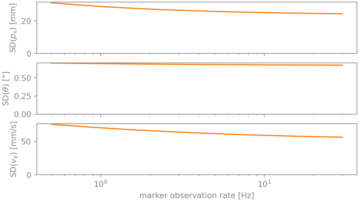
If we see the marker more often, then our position estimate must improve, no? Let’s see. Figure 2 plots the root variance on \(p_x\) for an observation rate ranging from 0.5 to 30 Hz:

As expected, the improvement is definitely there, though small it is: just 22 %. What is happening here? To uncover this, first have a look at \(\mathbf{R}\). The observation uncertainty on the markers relative x-axis position is only 3.1 mm, a fraction of the drone’s position uncertainty. The root challenge here is that that the relative observation has to be transformed to the world frame, and here the drone’s attitude \(\theta\) comes into play. Or actually, its covariance, as any uncertainty on it increases the uncertainty on the result. The orientation uncertainty is 0.71 ° - at a distance of 2.0 m, that makes for an uncertainty of 25 mm. Put differently, the position uncertainty is almost completely due to attitude uncertainty, and not due to the marker observation (which is already close to perfect). Camera improvements, such as executing more observations or increasing resolution, hence fail to add significant value.

Use marker orientation?

Given the attitude uncertainty, an additional observer would be welcome. A view on a visual marker such as an AprilTag provides both position and orientation, hence why not use it? The issue here lies in the variance magnitudes. Marker detection precision is in the order of several degrees, and that is considerably higher than the drone’s attitude uncertainty. Therefore, the marker orientation carries little relevant information. (An exception would be if the marker observation rate would be sufficiently high to average out the orientation noise, but in practice the required rate tends to be higher than what the drone’s processing units are capable of.)

So let’s go for a more stable gyro, then?

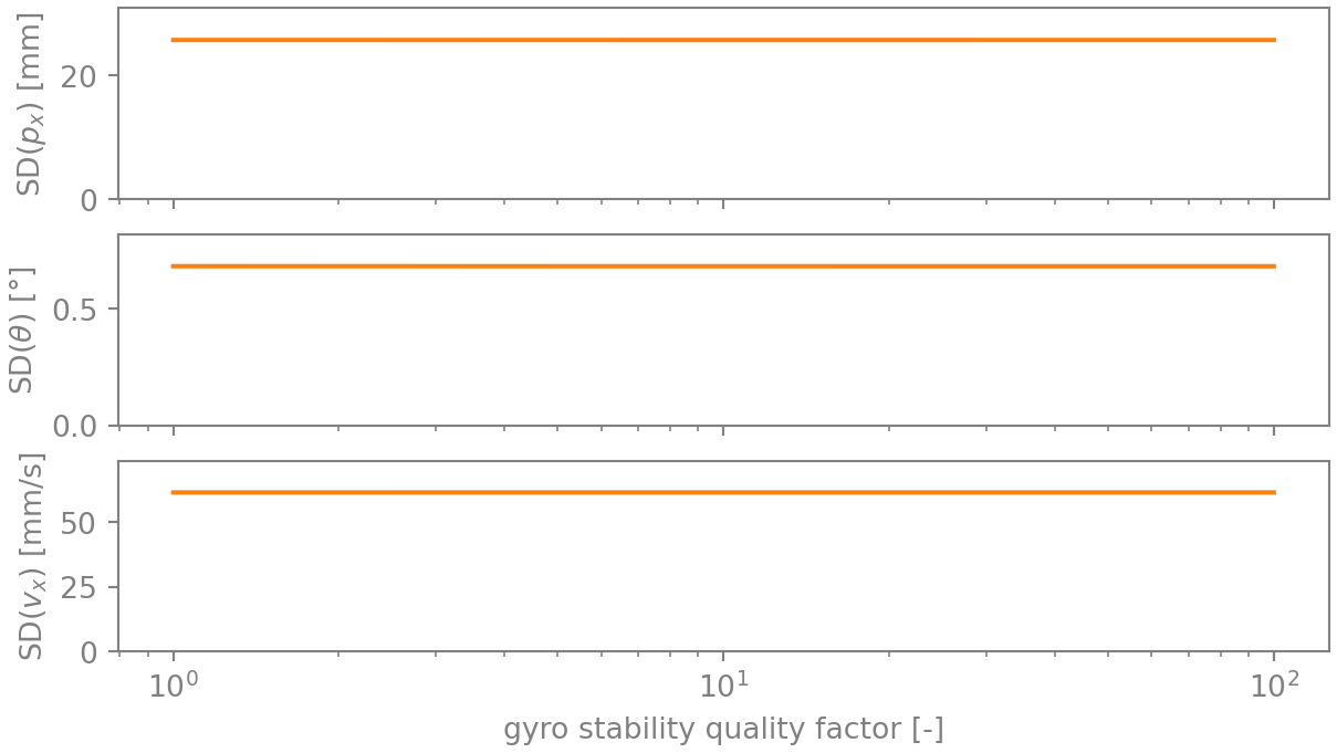
A basic characterization of a gyro or accelerometer consists of two values: measurement noise and bias drift velocity. The better IMUs have a built-in heater that maintains the sensor at constant temperature, as the bias drift velocity is temperature dependent. The result is a gyro that is more stable. Figure 3 shows what difference a 100-fold more stable gyro makes for this case: close to negligible. The reason for this is simple: the bias is easily estimated anyway, so improving that estimate even further by decreasing the rate of change yields diminished returns.

Does reducing gyro or accelerometer noise help?

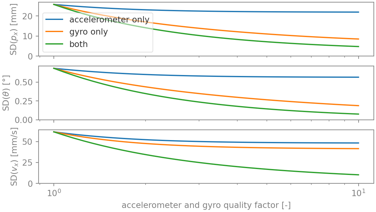
The two remaining parameters are then the gyro and accelerometer observation noises. Intuitively, it may seem that the latter is the most determining; after all, velocity and position are integrals of acceleration. On the other hand, lower gyro noise improves the attitude estimate, in turn reducing the uncertainty on the transformed marker position. Figure 4 graphs the effect - and it’s a bit of both: for \(p_x\), it’s the gyro that rules, while for \(v_x\), both are necessary to obtain a substantial improvement.

The latter result is particularly interesting. A better gyro on its own improves the attitude, but the velocity uncertainty remains high because of the noisy acceleration measurements (which effectively results in the velocity being estimated from the position observations). Meanwhile, only improving the accelerometer doesn’t yield gains as it doesn’t help in curbing the attitude uncertainty.

Conclusion: the way forward is to go for an IMU with a less noisy gyro and accelerometer.

Conclusion

Through this exploration of sensor fusion for autonomous multirotor landing, we unveiled insights that streamline the design of state estimation systems. Writing out the system matrices, converting discrete measurements to continuous ones, and performing sensitivity analyses allowed us to obtain many of the design insights that otherwise require actually simulating the full filter.

The key takeaway here is that this approach allows to bypass extensive implementation and simulation, letting us zero in on what really matters in the design phase. It empowers engineers and researchers to quickly assess the impact of different sensor configurations and noise characteristics on state estimation accuracy, and as such enables informed decisions early in the development process.

Did you apply similar techniques? What would you like to see discussed next? Share in the comments!